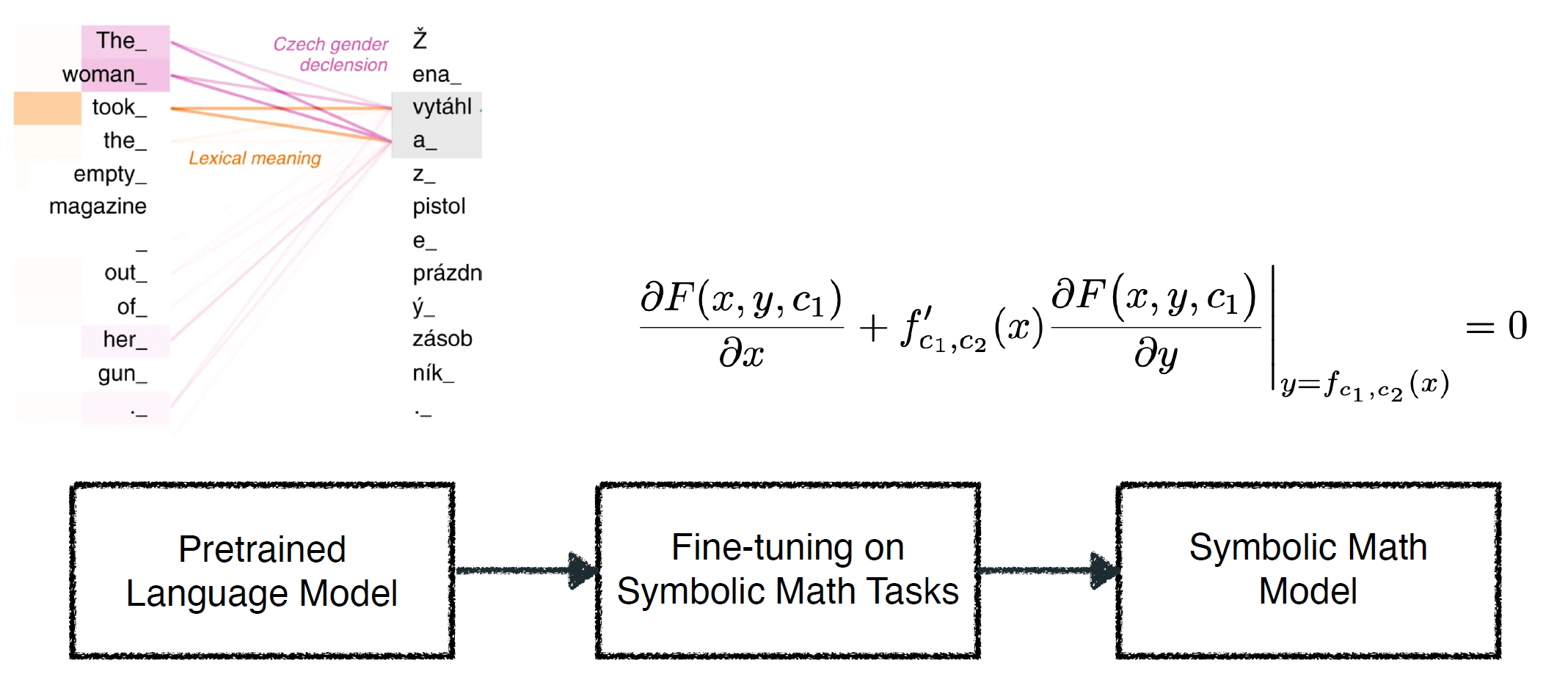
Solving symbolic mathematics has always been of in the arena of human ingenuity that needs compositional reasoning and recurrence. However, recent studies have shown that large-scale language models such as transformers are universal and surprisingly can be trained as a sequence-to-sequence task to solve complex mathematical equations. These large transformer models need humongous amounts of training data to generalize to unseen symbolic mathematics problems. In this work, we present a sample efficient way of solving the symbolic tasks by

1. Pretraining the transformer model with language translation and,
2. Fine-tuning the pretrained transformer model to solve the downstream task of symbolic mathematics.

We achieve comparable accuracy on the integration task with our pretrained model while using around 1.5 orders of magnitude less number of training samples with respect to the state-of-the-art deep learning for symbolic mathematics. The test accuracy on differential equation tasks is consider- ably lower comparing with integration as they need higher order recursions that are not present in language translations. We pretrain our model with different pairs of language translations. Our results show language bias in solving symbolic mathematics tasks. Finally, we study the robustness of the fine-tuned model on symbolic math tasks against distribution shift, and our approach generalizes better in distribution shift scenarios for the function integration.

Empirical Evaluation

In orther to examine the transfer from language translation to solving symbolic math equations and attempt to understand better why this happens and which factors enable this transfer, we desighn the following research questions. we refer to Lample & Charton (2019)’s model results with the keyword LC in our tables and visualizations.

i. Does this pretrained model help us to use less data for training?

As studied in Lample & Charton (2019), to train transformer architecture on the symbolic math data, we need a vast amount of training data for each task to achieve the highest accuracies (in the order of 40 million to 80 million training samples for each task.). We can see in the following table that our model outperformed in the integration task, with a considerable gap from the LC model. But it cannot properly perform on the differential equation task, especially the second-order differential equations.

	Our Model	LC’s Model
Integration (FWD)	87.4	79.4
Integration (BWD)	92.2	83.4
Integration (IBP)	86.2	87.4
ODE 1	62.2	71.8
ODE 2	17.9	39.9

The following figure extends this exploration by running the same experiment for different orders of magnitude of training data (i.e., 10K, 100K, and 1M). Our fine-tuned model has higher accuracy in comparison to LC in all tasks and with different training sample sizes, except that in the differential equations the accuracy growth of our model suddenly gets lower than the LC model when using the 1 million samples for training.

ii. Are the results of such fine-tuning, language dependent?

We investigate whether different languages used to train our pretrained models impact the results of this transfer learning. The following table shows the evaluation of accuracy of our Marian-MT model (in percentage (%)) on the integration and differential equation solving for different pretrained languages. The highest accuracy is indicated by bold case in each row (task). We see that the language has no major impact on the results of this fine-tuning.

Language	English Romanian	English Greek	English Arabic	English French	English Spanish	Greek English	Arabic English	French English	Spanish English
Integration (FWD)	38.8	39.3	43.9	47.7	43.5	39.1	43.3	50.5	40.4
Integration (BWD)	67.8	69.5	71.3	71.4	70.4	69.1	69.3	71.2	69.9
Integration (IBP)	51.5	48.6	53.5	52.5	51.8	47.9	50.7	52.7	51.7
ODE 1	23.4	17.3	16.4	18.9	18.7	16.2	22.5	19.7	20.2
ODE 2	1.8	2.5	2.7	2.9	3.3	2.2	2.3	2.3	2.0

iii. How robust this fine-tuned model is with the distribution shift?

It is important to see whether these transformer models are biased towards the distribution of their training data or not. In order to evaluate this concept, we define two different kinds of distribution shift as follows:

• The first one is only for the integration task and is similar to section 4.7 described in Lample & Charton (2019). Meaning that we will investigate how robust our models trained in section i are when we change their testing distribution. We report the evaluation metrics trained and tested on a different combination of training datasets in the following table:

  	Forward	Forward	Backward	Backward	Integration by parts	Integration by parts
  Data	Ours(mBart)	LC	Ours(mBart	LC	Ours(mBart)	LC
  FWD	87.38	79.42	7.30	6.90	74.20	74.10
  BWD	12.82	9.28	92.24	83.40	24.02	17.60
  IBP	30.46	28.70	35.00	20.50	86.26	87.44

• The second kind of distribution shift that we are interested in is due to the modality of the test dataset. This type of distribution shift was not studied by Lample & Charton (2019) and is a new type of distribution shifts we introduce in this paper. Each training sample we use on all tasks (in sections i and and ii) has a combination of all different types of equations such as polynomial, trigonometric, and logarithmic expressions. We want to see whether a model trained on this type of dataset can generalize to solve type-dominant functions (i.e, functions containing only polynomial equations or containing only trigonometric equations and so on.). Therefore, we generate different types of test data, varying in the kind of equation they represent, such as trigonometric equations, polynomial equations, and logarithmic equations (you can download this type-variant dataset from here). The results are reported in the following table:

  Testset Type	Metrics	Integration(FWD)	Integration(BWD)	Integration (IBP)	ODE 1	ODE 2
  Polynomials	Ours	60.6	67.8	70.7	39.1	8.9
  	LC	54.7	60.0	80.1	60.6	57.9
  Trigonometric	Ours	91.9	87.0	78.9	48.3	10.6
  	LC	92.4	85.8	91.8	74.4	60.6
  Logarithmic	Ours	90.9	75.1	72.4	35.9	6.8
  	LC	87.9	73.3	88.0	75.6	72.0

In order to have a better undrestanding of the results, we encourage the reader to read section 3 of the paper as well as the discussions in the 5th section of the paper.

Our Team

Please do not hesitate to contact us in case you have any questions.

Kimia Noorbakhsh	Mahdi Sharifi	Modar Sulaiman
Sharif University of Technology	University of South Carolina	University of Tartu

Kallol Roy	Pooyan Jamshidi
University of Tartu	University of South Carolina